DDPM前向过程
前向扩散指的是将一个复杂分布转换成简单分布的过程 T:Rd↦Rd,即:
x0∼pcomplex⟹T(x0)∼pprior
在DDPM中,将这个过程定义为马尔可夫链,通过不断地向复杂分布中的样本x0∼pcomplex添加高斯噪声。这个加噪过程可以表示为q(xt∣xt−1):
q(xt∣xt−1)xt=N(xt;1−βtxt−1,βtI)=1−βtxt−1+βtϵϵ∼N(0,I)
其中,{βt∈(0,1)}t=1T,是超参数。
从x0开始,不断地应用q(xt∣xt−1),经过足够大的T步加噪之后,最终得到纯噪声xT:
x0∼pcomplex→x1→⋯xt→⋯→xT∼pprior
除了迭代地使用q(xt∣xt−1)外,还可以使用q(xt∣x0)=N(xt;αˉtx0,(1−αˉt)I)一步到位,证明如下(两个高斯变量的线性组合仍然是高斯变量):
xt=αtxt−1+1−αtϵt−1=αtαt−1xt−2+1−αtαt−1ϵˉt−2=…=αˉtx0+1−αˉtϵ ;αt=1−αt ;ϵ∼N(0,I),αˉt=i=1∏tαi
一般来说,超参数βt的设置满足0<β1<⋯<βT<1,则αˉ1>⋯>αˉT→1,则xT会只保留纯噪声部分。
DDPM逆向过程
在前向扩散过程中,实现了:
x0∼pcomplex→x1→⋯xt→⋯→xT∼pprior
如果能够实现将前向扩散过程反转,也就实现了从简单分布到复杂分布的映射。逆向扩散过程则是将前向过程反转,实现从简单分布随机采样样本,迭代地使用q(xt−1∣xt),最终生成复杂分布的样本,即:
xT∼pprior→xT−1→⋯xt→⋯→x0∼pcomplex
为了求取q(xt−1∣xt),使用贝叶斯公式:
q(xt−1∣xt)=q(xt)q(xt∣xt−1)q(xt−1)
然而,公式中q(xt−1)和q(xt)不好求,根据DDPM的马尔科夫假设,可以为q(xt−1∣xt)添加条件(可以证明,如果向扩散过程中的βt足够小,那么q(xt−1∣xt)是高斯分布。):
q(xt−1∣xt)=q(xt−1∣xt,x0)=q(xt∣x0)q(xt∣xt−1,x0)q(xt−1∣x0)=q(xt∣x0)q(xt∣xt−1)q(xt−1∣x0)=N(xt−1;μ(xt;θ),σt2I)
其中,μ(xt;θ)是高斯分布的均值,σt可以用超参数表示:
μ(xt;θ)σt=1−αˉtαt(1−αˉt−1)xt+1−αˉtαˉt−1βtx0=1−αˉt1−αˉt−1⋅βt
式中x0可以反用公式xt=αˉtx0+1−αˉtϵt:
x0=αˉt1(xt−1−αˉtϵt)
则:
μ(xt;θ)=1−αˉtαt(1−αˉt−1)xt+1−αˉtαˉt−1βtx0=1−αˉtαt(1−αˉt−1)xt+1−αˉtαˉt−1βtαˉt1(xt−1−αˉtϵt)=αt1(xt−1−αˉt1−αtϵt)
而在推理的时候,ϵt是未知的,所以使用神经网络进行预测。综上,逆向扩散过程:
q(xt−1∣xt)xt−1=N(xt−1;μ(xt;θ),σt2I)=N(xt−1;αt1(xt−1−αˉt1−αtϵθ(xt,t)),(1−αˉt1−αˉt−1⋅βt)2I)=αt1(xt−1−αˉt1−αtϵθ(xt,t))+1−αˉt1−αˉt−1βt⋅ϵϵ∼N(0,I)
DDPM训练方法
DDPM的训练目标是最小化训练数据的负对数似然:
−logpθ(x0)≤−logpθ(x0)+KL(q(x1:T∣x0)∥pθ(x1:T∣x0))=−logpθ(x0)+Ex1:T∼q(x1:T∣x0)[logpθ(x0:T)/pθ(x0)q(x1:T∣x0)]=−logpθ(x0)+Ex1:T∼q(x1:T∣x0)[logpθ(x0:T)q(x1:T∣x0)+logpθ(x0)]=Ex1:T∼q(x1:T∣x0)[logpθ(x0:T)q(x1:T∣x0)] ;KL(⋅∥⋅)≥0 ;pθ(x1:T∣x0)=pθ(x0)pθ(x0:T)
其中pθ(x1:T∣x0)是使用网络估计分布q(变分推断),定义LVLB≜Eq(x0:T)[logpθ(x0:T)q(x1:T∣x0)]≥−Eq(x0)logpθ(x0),那么VLB是训练数据的负对数似然的上节,最小化VLB就是最小化负对数似然。继续对VLB拆分:
LVLB=Eq(x0:T)[logpθ(x0:T)q(x1:T∣x0)]=Eq[logpθ(xT)∏t=1Tpθ(xt−1∣xt)∏t=1Tq(xt∣xt−1)]=Eq[−logpθ(xT)+t=1∑Tlogpθ(xt−1∣xt)q(xt∣xt−1)]=Eq[−logpθ(xT)+t=2∑Tlogpθ(xt−1∣xt)q(xt∣xt−1)+logpθ(x0∣x1)q(x1∣x0)]=Eq[−logpθ(xT)+t=2∑Tlogpθ(xt−1∣xt)q(xt∣xt−1,x0)+logpθ(x0∣x1)q(x1∣x0)]=Eq[−logpθ(xT)+t=2∑Tlog(pθ(xt−1∣xt)q(xt−1∣xt,x0)q(xt−1∣x0)q(xt∣x0))+logpθ(x0∣x1)q(x1∣x0)]=Eq[logpθ(xT)q(xT∣x0)+t=2∑Tlogpθ(xt−1∣xt)q(xt−1∣xt,x0)−logpθ(x0∣x1)]=EqLTKL(q(xT∣x0)∥pθ(xT))+t=2∑TLt−1KL(q(xt−1∣xt,x0)∥pθ(xt−1∣xt))−L0logpθ(x0∣x1)=Eq[LT+t=2∑TLt−1−L0] ;q(xt∣xt−1)=q(xt∣xt−1,x0) ;Bayes Theorem
- 由于xT是纯噪声,所以LT是常数
- 对于L0,DDPM专门设计了特殊的pθ(x0∣x1)
- 对于Lt≜KL(q(xt∣xt+1,x0)∥pθ(xt∣xt+1))1≤t≤T−1,是两个正态分布的KL散度,有解析解。在DDPM中,使用了简化之后的损失函数:
Ltsimple=Et∼[1,T],x0,ϵt[∥ϵt−ϵθ(αˉtx0+1−αˉtϵt,t)∥22]
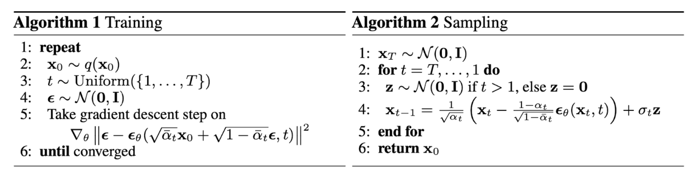
DDPM总结
综上,DDPM的训练和采样/推理过程如下图所示:
扩散模型与分数生成模型的联系
对于分数:∇xlogp(x)=∇x[−2σ21(x−μ)2]=−σx−μ=−σ2(μ+σϵ)−μ=−σϵ
又因为:xt=αˉtx0+1−αˉtϵ, ϵ∼N(0,1)
所以:
∇xtlog p(xt)=Ep(x0)[log p(xt∣x0)]=−1−αˉtϵθ(xt,t)
因此,扩散模型的噪声估计器和score只相差一个scale:−1−αˉt1.
分类器引导采样
为了让扩散模型能够进行条件生成,需要建模数据与条件的联合分布,换句话说,需要让模型估计这个联合分布的score:
=∇xt[log(p(y∣xt)p(xt))]=∇xt[logp(y∣xt)+logp(xt)]=∇xtlog p(y∣xt)+∇xtlog p(xt)
p(y∣xt)是一个分类器,训练这样一个分类器去估计这一项
=∇xtlog p(y∣xt)+∇xtlog p(xt)≈ ∇xtlog fϕ(y∣xt)−1−αˉt1ϵθ(xt,t)
这样就得到了一个新的score估计器:
∇xtlog p(xt,y)=−1−αˉt1ϵ~θ(xt,y,t)=∇xtlog fϕ(y∣xt)−1−αˉt1ϵθ(xt,t)⇔ ϵ~θ(xt,t,y)=ϵθ(xt,t,y)−1−αˉt∇xtlog fϕ(y∣xt)
为了设置分类器的引导强度,新增一个引导参数w:
ϵ~θ(xt,t,y)=ϵθ(xt,t,y)−w1−αˉt∇xtlogfϕ(y∣xt)
无分类器引导采样
在分类器引导采样中,根据贝叶斯公式:
∇xtlog p(y∣xt)=∇xtlog[p(xt)p(xt∣y)p(y)]=∇xtlog p(xt∣y)+∇xtlog p(y) − ∇xtlog p(xt)=∇xtlog p(xt∣y)−∇xtlog p(xt)=−1−αˉt1(ϵ(xt,t,y)−ϵ(xt,t))
代入分类器引导采样公式中:
ϵ~θ(xt,t,y)=ϵθ(xt,t,y)−w1−αˉt∇xtlogfϕ(y∣xt)=ϵθ(xt,t,y)+w[ϵ(xt,t,y)−ϵ(xt,t)]
即,分类器引导采样中分类器提供的方向等价为ϵ(xt,t,y)−ϵ(xt,t),这个方向靠近条件的方向,远离无条件方向
思考
进一步思考,这一项的数值大小ϵ(xt,t,y)−ϵ(xt,t)标志着数据和条件对齐的程度,这是一个隐式的分类器,能够利用这个特点分类
继续进一步,如果将无条件score估计网络ϵ(xt,t)换成另一个条件y′,即ϵ(xt,t,y′)。则:
ϵ(xt,t,y)−ϵ(xt,t,y′)=[ϵ(xt,t,y)−ϵ(xt,t)]−[ϵ(xt,t,y′)−ϵ(xt,t)]
这里出现了两个隐式分类器,第一个是衡量数据和条件y的对齐程度,第二个是衡量数据和条件y′的对齐程度。如果使用这两个隐式分类器替换之前的隐式分类器,那么就相当于在生成过程中让数据尽可能对齐条件y,远离y′,这个做法被广泛用于Stable Diffusion中(negative prompt),negative prompt一般被设置为low quality, ugly等想让模型远离提示词。既然都能够同时使用1个正提示词和1个负提示词进行引导,那么也可以实现m个提示词(隐式分类器)进行引导:
Compositional visual generation with composable diffusion models
无分类器引导中的CFG值
无分类器引导采样中的w一般被称为CFG值,越大表示越向条件靠近(可以提高样本的保真度),越小表示越向非条件靠近(可以提高样本的多样性),可以根据实际需求调节。
BTW,虽然扩散模型可以像cGAN或cVAE那样训练一个conditional model,即ϵ(xt,t,y),这个在条件y较简单的时候(例如只是一个类别标签),一个好的backbone仍然能够实现条件生成。但是当条件变复杂的时候(例如文本,草图等),无分类器引导采样就变得很重要了,这个是目前非常主流的做法。
Reference
- 从零开始了解Diffusion Models
- https://ayandas.me/blog-tut/2021/12/04/diffusion-prob-models.html
- What are Diffusion Models
- An introduction to Diffusion Probabilistic Models